Modeling and Outputs

This article covers the tidy result layer, filtering, plots, and export.

It also shows how the package supports the comparison logic used in the companion paper, Wrapping input-output multipliers in confidence intervals. The key idea is to keep Leontief benchmark results and SUBE model outputs in a shared comparison structure instead of treating them as separate reporting pipelines.

The examples below use shipped sample data, but the modeling and output layer works identically for any SUT source once data is in the canonical long format - whether it came from WIOD, FIGARO, or a custom national supply-use table. Data preparation and format details are covered in the data-preparation vignette.

Compute the sample workflow

bundle <- build_matrices(
  extract_domestic_block(sube_example_data("sut_data")),
  sube_example_data("cpa_map"),
  sube_example_data("ind_map")
)
result <- compute_sube(bundle, sube_example_data("inputs"))
head(result$tidy)
#>     YEAR COUNTRY CPAagg variable     value    measure     type
#>    <int>  <char> <char>   <fctr>     <num>     <char>   <char>
#> 1:  2020     AAA    P01       GO 1.6250000 multiplier leontief
#> 2:  2020     AAA    P02       GO 1.4285714 multiplier leontief
#> 3:  2020     AAA    P01       VA 0.5416667 multiplier leontief
#> 4:  2020     AAA    P02       VA 0.4761905 multiplier leontief
#> 5:  2020     AAA    P01      EMP 0.3993056 multiplier leontief
#> 6:  2020     AAA    P02      EMP 0.3214286 multiplier leontief

Filter and plot

filtered <- filter_sube(result$tidy)
plot_sube(filtered, by = "country", kind = "boxplot", measure = "multiplier")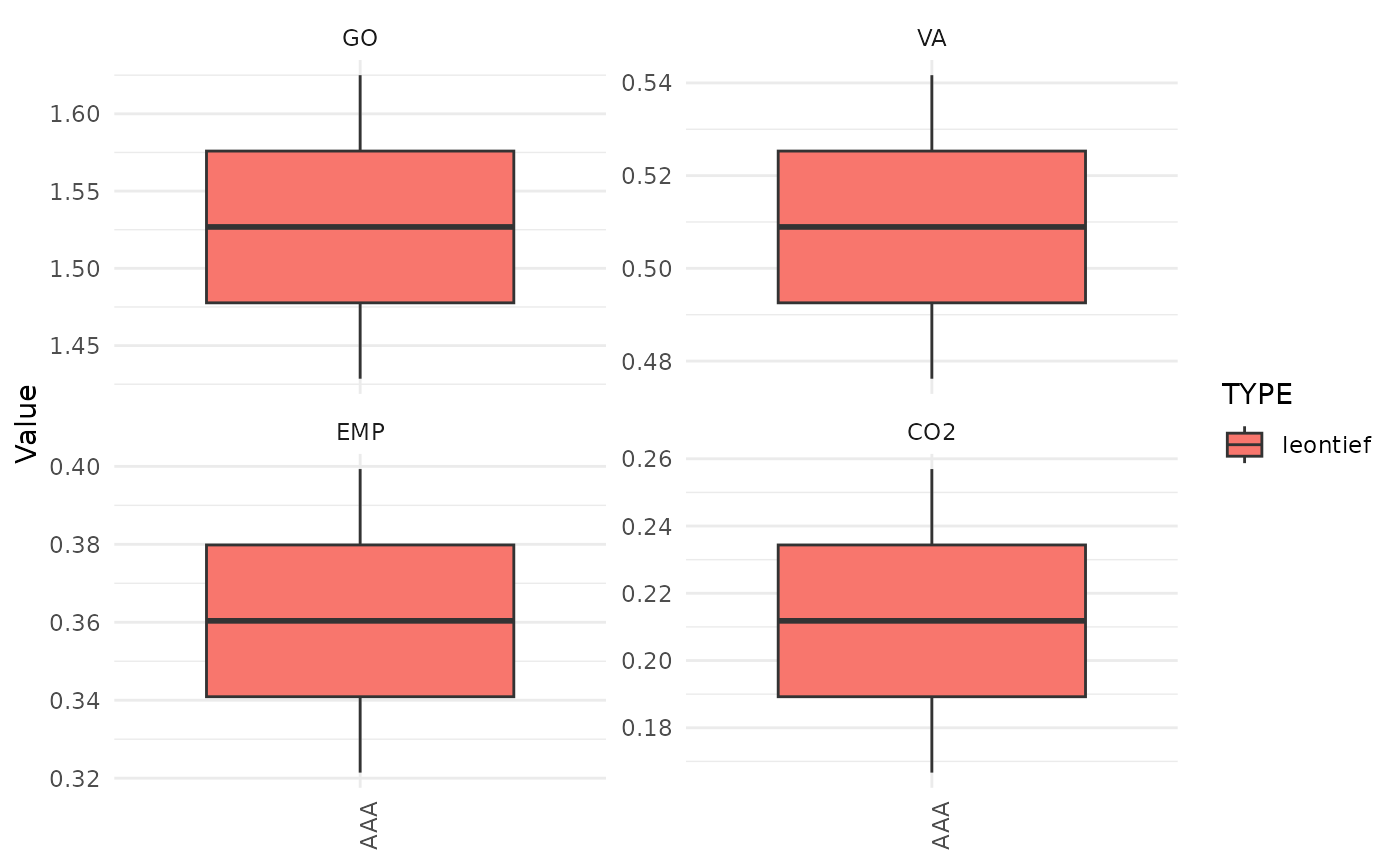

Paper-style comparison plots

models <- estimate_elasticities(
  sube_example_data("model_data"),
  predictor_vars = c("P01", "P02")
)
#> Warning in qt(a, object$df.residual): NaNs produced
#> Warning in qt(a, object$df.residual): NaNs produced
#> Warning in qt(a, object$df.residual): NaNs produced
#> Warning in qt(a, object$df.residual): NaNs produced
#> Warning in qt(a, object$df.residual): NaNs produced
#> Warning in qt(a, object$df.residual): NaNs produced
#> Warning in qt(a, object$df.residual): NaNs produced
#> Warning in qt(a, object$df.residual): NaNs produced
#> Warning in qt(a, object$df.residual): NaNs produced
#> Warning in qt(a, object$df.residual): NaNs produced
#> Warning in qt(a, object$df.residual): NaNs produced
#> Warning in qt(a, object$df.residual): NaNs produced
#> Warning in qt(a, object$df.residual): NaNs produced
#> Warning in qt(a, object$df.residual): NaNs produced
#> Warning in qt(a, object$df.residual): NaNs produced
#> Warning in qt(a, object$df.residual): NaNs produced
#> Warning in summary.lm(x): essentially perfect fit: summary may be unreliable
#> Warning in summary.lm(object, ...): essentially perfect fit: summary may be
#> unreliable
#> Warning in summary.lm(object, ...): essentially perfect fit: summary may be
#> unreliable
#> Warning in summary.lm(x): essentially perfect fit: summary may be unreliable
#> Warning in summary.lm(object, ...): essentially perfect fit: summary may be
#> unreliable
#> Warning in summary.lm(object, ...): essentially perfect fit: summary may be
#> unreliable
#> Warning in summary.lm(x): essentially perfect fit: summary may be unreliable
#> Warning in summary.lm(object, ...): essentially perfect fit: summary may be
#> unreliable
#> Warning in summary.lm(object, ...): essentially perfect fit: summary may be
#> unreliable
#> Warning in summary.lm(x): essentially perfect fit: summary may be unreliable
#> Warning in summary.lm(object, ...): essentially perfect fit: summary may be
#> unreliable
#> Warning in summary.lm(object, ...): essentially perfect fit: summary may be
#> unreliable
#> Warning in qt(a, object$df.residual): NaNs produced
#> Warning in qt(a, object$df.residual): NaNs produced
#> Warning in qt(a, object$df.residual): NaNs produced
#> Warning in qt(a, object$df.residual): NaNs produced
#> Warning in qt(a, object$df.residual): NaNs produced
#> Warning in qt(a, object$df.residual): NaNs produced
#> Warning in qt(a, object$df.residual): NaNs produced
#> Warning in qt(a, object$df.residual): NaNs produced
#> Warning in summary.lm(object, ...): essentially perfect fit: summary may be
#> unreliable
#> Warning in summary.lm(object, ...): essentially perfect fit: summary may be
#> unreliable
#> Warning in summary.lm(object, ...): essentially perfect fit: summary may be
#> unreliable
#> Warning in summary.lm(object, ...): essentially perfect fit: summary may be
#> unreliable
#> Warning in summary.lm(object, ...): essentially perfect fit: summary may be
#> unreliable
#> Warning in summary.lm(object, ...): essentially perfect fit: summary may be
#> unreliable
#> Warning in summary.lm(object, ...): essentially perfect fit: summary may be
#> unreliable
#> Warning in summary.lm(object, ...): essentially perfect fit: summary may be
#> unreliable

comparison <- prepare_sube_comparison(
  result,
  models,
  measure = "multiplier",
  variables = c("GO", "VA")
)

leontief_long <- extract_leontief_matrices(result, matrix = "L", format = "long")
head(leontief_long)
#>    COUNTRY  YEAR matrix    row    col     value
#>     <char> <int> <char> <char> <char>     <num>
#> 1:     AAA  2020      L    P01    P01 1.3750000
#> 2:     AAA  2020      L    P02    P01 0.2500000
#> 3:     AAA  2020      L    P01    P02 0.1428571
#> 4:     AAA  2020      L    P02    P02 1.2857143

names(plot_paper_comparison(
  comparison,
  kind = "by_country",
  measure = "multiplier",
  variables = "GO"
))
#> [1] "Leontief" "ols"      "pooled"   "between"

extract_leontief_matrices() also supports format = "list" and format = "wide" when you want matrix-oriented outputs instead of the tidy long table used by most comparison helpers.

These helpers are designed for the same kinds of questions emphasized in the paper: where Leontief and econometric estimates line up, where they diverge, and how those differences vary across countries and products.

Export

write_sube("outputs/final_results", filtered, format = "csv")
write_sube(
  "outputs/comparison_bundle",
  list(filtered = filtered, summary = result$summary),
  format = "csv"
)

A single table writes to one normalized file path. A named list writes one file per entry into the target directory, which is useful for comparison-ready bundles.

Model estimation tables

models <- estimate_elasticities(
  sube_example_data("model_data"),
  predictor_vars = c("P01", "P02")
)
#> Warning in qt(a, object$df.residual): NaNs produced
#> Warning in qt(a, object$df.residual): NaNs produced
#> Warning in qt(a, object$df.residual): NaNs produced
#> Warning in qt(a, object$df.residual): NaNs produced
#> Warning in qt(a, object$df.residual): NaNs produced
#> Warning in qt(a, object$df.residual): NaNs produced
#> Warning in qt(a, object$df.residual): NaNs produced
#> Warning in qt(a, object$df.residual): NaNs produced
#> Warning in qt(a, object$df.residual): NaNs produced
#> Warning in qt(a, object$df.residual): NaNs produced
#> Warning in qt(a, object$df.residual): NaNs produced
#> Warning in qt(a, object$df.residual): NaNs produced
#> Warning in qt(a, object$df.residual): NaNs produced
#> Warning in qt(a, object$df.residual): NaNs produced
#> Warning in qt(a, object$df.residual): NaNs produced
#> Warning in qt(a, object$df.residual): NaNs produced
#> Warning in summary.lm(x): essentially perfect fit: summary may be unreliable
#> Warning in summary.lm(object, ...): essentially perfect fit: summary may be
#> unreliable
#> Warning in summary.lm(object, ...): essentially perfect fit: summary may be
#> unreliable
#> Warning in summary.lm(x): essentially perfect fit: summary may be unreliable
#> Warning in summary.lm(object, ...): essentially perfect fit: summary may be
#> unreliable
#> Warning in summary.lm(object, ...): essentially perfect fit: summary may be
#> unreliable
#> Warning in summary.lm(x): essentially perfect fit: summary may be unreliable
#> Warning in summary.lm(object, ...): essentially perfect fit: summary may be
#> unreliable
#> Warning in summary.lm(object, ...): essentially perfect fit: summary may be
#> unreliable
#> Warning in summary.lm(x): essentially perfect fit: summary may be unreliable
#> Warning in summary.lm(object, ...): essentially perfect fit: summary may be
#> unreliable
#> Warning in summary.lm(object, ...): essentially perfect fit: summary may be
#> unreliable
#> Warning in qt(a, object$df.residual): NaNs produced
#> Warning in qt(a, object$df.residual): NaNs produced
#> Warning in qt(a, object$df.residual): NaNs produced
#> Warning in qt(a, object$df.residual): NaNs produced
#> Warning in qt(a, object$df.residual): NaNs produced
#> Warning in qt(a, object$df.residual): NaNs produced
#> Warning in qt(a, object$df.residual): NaNs produced
#> Warning in qt(a, object$df.residual): NaNs produced
#> Warning in summary.lm(object, ...): essentially perfect fit: summary may be
#> unreliable
#> Warning in summary.lm(object, ...): essentially perfect fit: summary may be
#> unreliable
#> Warning in summary.lm(object, ...): essentially perfect fit: summary may be
#> unreliable
#> Warning in summary.lm(object, ...): essentially perfect fit: summary may be
#> unreliable
#> Warning in summary.lm(object, ...): essentially perfect fit: summary may be
#> unreliable
#> Warning in summary.lm(object, ...): essentially perfect fit: summary may be
#> unreliable
#> Warning in summary.lm(object, ...): essentially perfect fit: summary may be
#> unreliable
#> Warning in summary.lm(object, ...): essentially perfect fit: summary may be
#> unreliable
head(models$pooled)
#>      term estimate    std.error    statistic      p.value   lwr   upr  mean
#>    <char>    <num>        <num>        <num>        <num> <num> <num> <num>
#> 1:    P01      2.0 3.723801e-16 5.370856e+15 3.466674e-32   2.0   2.0     2
#> 2:    P02      1.0 3.723801e-16 2.685428e+15 1.386670e-31   1.0   1.0     2
#> 3:    P01      0.5 2.019515e-17 2.475842e+16 1.631376e-33   0.5   0.5     2
#> 4:    P02      0.2 2.019515e-17 9.903369e+15 1.019610e-32   0.2   0.2     2
#> 5:    P01      0.3 5.909454e-17 5.076612e+15 3.880182e-32   0.3   0.3     2
#> 6:    P02      0.1 5.909454e-17 1.692204e+15 3.492164e-31   0.1   0.1     2
#>    mean_y elasticity COUNTRY  YEAR      y   type
#>     <num>      <num>  <char> <int> <char> <char>
#> 1:    6.0  0.6666667     AAA    NA     GO pooled
#> 2:    6.0  0.3333333     AAA    NA     GO pooled
#> 3:    1.4  0.7142857     AAA    NA     VA pooled
#> 4:    1.4  0.2857143     AAA    NA     VA pooled
#> 5:    0.8  0.7500000     AAA    NA    EMP pooled
#> 6:    0.8  0.2500000     AAA    NA    EMP pooled

The comparison layer can also be used for regression-style and interval-range plots when the modeling results contain enough information. These helpers return named lists of ggplot objects keyed by the available model or variable selections in the supplied data:

paper_regression <- plot_paper_regression(
  comparison,
  method = "between",
  measure = "multiplier",
  variables = "GO"
)

interval_ranges <- plot_paper_interval_ranges(
  models,
  by = "country",
  variables = "GO"
)