Post-estimation Analysis with bsvarPost

This article follows one fiscal analysis from posterior draws to an exported comparison table. It assumes familiarity with R and structural VARs. The demo models use bsvars default identification; economic shock interpretations must follow the restrictions used in your own model.

Load the demonstration models

library(bsvarPost)
post <- readRDS(system.file("extdata", "fiscal_post_bsvar.rds",
  package = "bsvarPost", mustWork = TRUE))
post_alt <- readRDS(system.file("extdata", "fiscal_post_bsvar_alt.rds",
  package = "bsvarPost", mustWork = TRUE))
metadata <- read.csv(system.file("extdata", "demo-metadata.csv",
  package = "bsvarPost", mustWork = TRUE))
metadata[1:2, c("file", "p", "seed", "draws", "sample_start", "sample_end")]
#>                        file p seed draws sample_start sample_end
#> 1     fiscal_post_bsvar.rds 1  123   200         1948       2026
#> 2 fiscal_post_bsvar_alt.rds 3  456   200         1948       2026

The baseline has one lag and the alternative three. Both contain 200 retained draws, a small demonstration sample rather than evidence of sampling adequacy. The installed metadata records estimation software versions, transformations, sample ranges and checksums. The frozen input data travel with these fits. Results obtained by re-estimating may differ across software versions.

GDP’s response to government spending

responses <- tidy_irf(post, horizon = 12, probability = 0.90)
gdp_irf <- subset(responses, variable == "gdp" & shock == "gs")
gdp_irf[gdp_irf$horizon %in% c(0, 4, 8, 12),
  c("horizon", "median", "lower", "upper")]
#> # A tibble: 4 × 4
#>   horizon     median    lower    upper
#>     <dbl>      <dbl>    <dbl>    <dbl>
#> 1       0 -0.0000337 -0.00207 0.00112 
#> 2       4 -0.000686  -0.00222 0.000949
#> 3       8 -0.00117   -0.00306 0.00101 
#> 4      12 -0.00160   -0.00410 0.00114

Horizon zero is impact; horizon 12 is twelve quarters later, giving thirteen reported horizons. Bounds are pointwise 90% equal-tailed credible intervals, not a simultaneous band over the entire path. The response is in the data’s log units under the fitted structural-shock normalization. It is not implicitly normalized to a one-dollar or one-percent spending increase.

Cumulative responses and units

For draw $s$, the cumulative response through horizon $H$ is

$$C^{(s)}_{ij}(H) = \sum_{h=0}^{H} IRF^{(s)}_{ij}(h).$$

Summation happens within each draw, before posterior summaries are computed. The cumulative posterior median need not equal the sum of marginal medians.

cumulative <- tidy_cdm(post, horizon = 12, probability = 0.90)
gdp_cdm <- subset(cumulative, variable == "gdp" & shock == "gs")
gdp_cdm[gdp_cdm$horizon %in% c(0, 4, 8, 12),
  c("horizon", "median", "lower", "upper", "scale_by", "scale_factor")]
#> # A tibble: 4 × 6
#>   horizon     median    lower   upper scale_by scale_factor
#>     <dbl>      <dbl>    <dbl>   <dbl> <chr>           <dbl>
#> 1       0 -0.0000337 -0.00207 0.00112 none                1
#> 2       4 -0.00175   -0.00998 0.00487 none                1
#> 3       8 -0.00587   -0.0190  0.00880 none                1
#> 4      12 -0.0104    -0.0318  0.0131  none                1

These inputs are log real per capita levels, without multiplication by 100. For example, an IRF of 0.001 log units is approximately a 0.1% change (exactly 100 * (exp(0.001) - 1) percent). For one hypothetical draw with responses 0.001, 0.002, and 0.001, the cumulative response at horizon 2 is 0.004 log units summed across three quarters. This is not the endpoint percentage change or a dollar-per-dollar fiscal multiplier.

example_irf <- c(0.001, 0.002, 0.001)
c(impact_percent = 100 * expm1(example_irf[1]),
  cumulative_log_response = sum(example_irf))
#>          impact_percent cumulative_log_response 
#>                 0.10005                 0.00400
scaled <- tidy_cdm(post, horizon = 12, probability = 0.90,
  scale_by = "shock_sd", scale_var = "gs")
subset(scaled, variable == "gdp" & shock == "gs" & horizon == 12,
  select = c(median, scale_by, scale_var, scale_factor))
#> # A tibble: 1 × 4
#>    median scale_by scale_var scale_factor
#>     <dbl> <chr>    <chr>            <dbl>
#> 1 -0.0589 shock_sd gs               0.177

shock_sd divides each cumulative response by the reported sample standard deviation of the selected observed variable (gs here). It does not set the shock’s impact spending response to one. A fiscal multiplier requires the output and spending responses expressed in compatible levels and their appropriate cumulative ratio. The package does not infer that conversion from these log series. See ?cdm and ?posterior_provenance in R.

figure <- ggplot2::autoplot(gdp_cdm) +
  ggplot2::labs(x = "Quarters after shock", y = "Cumulative log response")

GDP response to the gs shock, summed from impact through each horizon. Line: posterior median; ribbon: pointwise 90% equal-tailed interval. Original log units; no additional scaling.

Compare lag specifications

comparison <- compare_cdm(baseline = post, longer_lag = post_alt,
  horizon = 12, probability = 0.90)
comparison_gdp <- subset(comparison, variable == "gdp" & shock == "gs")
comparison_gdp[comparison_gdp$horizon %in% c(0, 4, 8, 12),
  c("model", "horizon", "median", "lower", "upper")]
#> # A tibble: 8 × 5
#>   model      horizon     median    lower    upper
#>   <chr>        <dbl>      <dbl>    <dbl>    <dbl>
#> 1 baseline         0 -0.0000337 -0.00207 0.00112 
#> 2 baseline         4 -0.00175   -0.00998 0.00487 
#> 3 baseline         8 -0.00587   -0.0190  0.00880 
#> 4 baseline        12 -0.0104    -0.0318  0.0131  
#> 5 longer_lag       0 -0.0000230 -0.00129 0.000971
#> 6 longer_lag       4 -0.00236   -0.0107  0.00617 
#> 7 longer_lag       8 -0.00925   -0.0289  0.0106  
#> 8 longer_lag      12 -0.0165    -0.0511  0.0139

The names identify models in tables and legends. This is a sensitivity comparison, not a model-selection criterion or a posterior probability that one model’s response exceeds the other’s.

figure <- ggplot2::autoplot(comparison_gdp) +
  ggplot2::labs(x = "Quarters after shock", y = "Cumulative log response")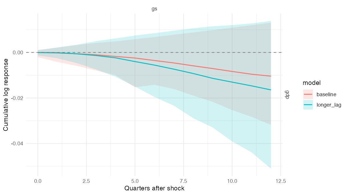

GDP cumulative response to gs: baseline p=1 and longer_lag p=3. Lines and ribbons show medians and pointwise 90% equal-tailed intervals in original log units, without additional scaling.

Select one representative draw

A path of marginal medians need not correspond to a single retained structural model. Select one draw closest to the GDP response’s median target over 0–12:

representative <- median_target_irf(post, horizon = 12, probability = 0.90,
  variables = "gdp", shocks = "gs", horizons = 0:12)
representative$draw_index
#> [1] 28
representative_path <- subset(summary(representative),
  variable == "gdp" & shock == "gs")
representative_path[representative_path$horizon %in% c(0, 4, 8, 12),
  c("horizon", "median", "draw_index", "selected_draw_id", "method")]
#> # A tibble: 4 × 5
#>   horizon    median draw_index selected_draw_id method       
#>     <dbl>     <dbl>      <int> <chr>            <chr>        
#> 1       0 -0.000121         28 28               median_target
#> 2       4 -0.000638         28 28               median_target
#> 3       8 -0.00113          28 28               median_target
#> 4      12 -0.00160          28 28               median_target

Here median is the selected draw’s response, not the posterior median. The selected draw provides a coherent model, not an uncertainty interval. The representative object retains the full array, so explicitly filter the plot to match the selected target:

figure <- ggplot2::ggplot(gdp_irf, ggplot2::aes(horizon, median)) +
  ggplot2::geom_ribbon(ggplot2::aes(ymin = lower, ymax = upper),
    fill = "#6baed6", alpha = 0.25) +
  ggplot2::geom_line(ggplot2::aes(colour = "Posterior median")) +
  ggplot2::geom_line(data = representative_path,
    ggplot2::aes(colour = "Selected draw")) +
  ggplot2::scale_colour_manual(values = c("Posterior median" = "#2171b5",
    "Selected draw" = "#cb181d")) +
  ggplot2::labs(x = "Quarters after shock", y = "GDP log response", colour = NULL) +
  ggplot2::theme_minimal()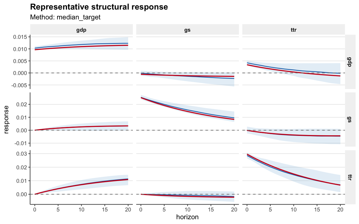

GDP IRF to gs in original log units. Red: one draw selected over this response at horizons 0–12. Blue: posterior median; ribbon: pointwise 90% equal-tailed interval. No additional scaling.

Export results with provenance

as_kable(comparison_gdp, preset = "compact", digits = 3,
  caption = "GDP cumulative response to government spending")

GDP cumulative response to government spending

Model	Variable	Shock	Horizon	Mean	Median	Lower	Upper
baseline	gdp	gs	0	-0.001	0.000	-0.002	0.001
baseline	gdp	gs	1	-0.001	0.000	-0.004	0.002
baseline	gdp	gs	2	-0.002	-0.001	-0.006	0.003
baseline	gdp	gs	3	-0.003	-0.001	-0.008	0.004
baseline	gdp	gs	4	-0.004	-0.002	-0.010	0.005
baseline	gdp	gs	5	-0.005	-0.002	-0.015	0.006
baseline	gdp	gs	6	-0.008	-0.004	-0.014	0.007
baseline	gdp	gs	7	-0.011	-0.005	-0.016	0.008
baseline	gdp	gs	8	-0.016	-0.006	-0.019	0.009
baseline	gdp	gs	9	-0.022	-0.007	-0.022	0.010
baseline	gdp	gs	10	-0.032	-0.008	-0.025	0.011
baseline	gdp	gs	11	-0.045	-0.010	-0.028	0.012
baseline	gdp	gs	12	-0.064	-0.010	-0.032	0.013
longer_lag	gdp	gs	0	-0.001	0.000	-0.001	0.001
longer_lag	gdp	gs	1	-0.003	0.000	-0.003	0.002
longer_lag	gdp	gs	2	-0.006	-0.001	-0.005	0.003
longer_lag	gdp	gs	3	-0.010	-0.001	-0.007	0.005
longer_lag	gdp	gs	4	-0.015	-0.002	-0.011	0.006
longer_lag	gdp	gs	5	-0.023	-0.004	-0.015	0.007
longer_lag	gdp	gs	6	-0.038	-0.006	-0.020	0.008
longer_lag	gdp	gs	7	-0.072	-0.007	-0.023	0.010
longer_lag	gdp	gs	8	-0.160	-0.009	-0.029	0.011
longer_lag	gdp	gs	9	-0.398	-0.011	-0.033	0.012
longer_lag	gdp	gs	10	-1.052	-0.013	-0.039	0.012
longer_lag	gdp	gs	11	-2.864	-0.015	-0.044	0.013
longer_lag	gdp	gs	12	-7.897	-0.016	-0.051	0.014

output <- tempfile(fileext = ".csv")
write_bsvar_csv(comparison_gdp, file = output)
exported <- read.csv(output, check.names = FALSE)
exported[1:2, c("Model", "Horizon", "Median", "Interval probability",
  "Interval method", "Scaling", "Source package", "Source version", "Draw count")]
#>      Model Horizon        Median Interval probability Interval method Scaling
#> 1 baseline       0 -3.370222e-05                  0.9    equal_tailed    none
#> 2 baseline       1 -2.287561e-04                  0.9    equal_tailed    none
#>   Source package Source version Draw count
#> 1         bsvars              4        200
#> 2         bsvars              4        200

Replace output with your chosen path to keep the file. The default export retains provenance with readable column labels; the compact table is for presentation. source_version identifies software used for the current calculation; estimation history is in the demo metadata. Economic units can be unknown because arbitrary transformations cannot be reconstructed from a posterior object.

For scripts that require fixed column names, select a schema explicitly and use the standard CSV writer:

schema <- c("model", "variable", "shock", "horizon", "median", "lower", "upper",
  "interval_probability", "interval_method", "scale_by", "scale_factor",
  "source_package", "source_version", "n_draws")
machine_output <- tempfile(fileext = ".csv")
write.csv(as.data.frame(comparison_gdp)[, schema], machine_output, row.names = FALSE)

Supported plotting inputs

ggplot2::autoplot() handles response summaries and supported draw-level paths; publish_bsvar_plot() adds publication styling for supported families. Individual timing summaries and draw-level hypothesis or event tables do not have an automatic plot. Summarize first or use a suitable comparison/family plot; passing unsupported inputs raises an explicit error.

probabilities <- hypothesis_irf(post, variables = "gdp", shocks = "gs",
  horizon = 0:12, relation = ">", value = 0)
probability_plot <- plot_hypothesis(probabilities)

For grouped historical decompositions, consult the draw-level input recipe.

Estimate your own models

This optional recipe uses the same frozen input, seeds and 200-draw settings as the demo generator. For research, choose an appropriate model, sampling length and diagnostic strategy; 200 draws is only an illustration.

fiscal_data <- readRDS(system.file("extdata", "us_fiscal_lsuw.rds",
  package = "bsvarPost", mustWork = TRUE))
set.seed(123)
spec <- bsvars::specify_bsvar$new(fiscal_data, p = 1)
post <- bsvars::estimate(spec, S = 200, thin = 1, show_progress = FALSE)
set.seed(456)
spec_alt <- bsvars::specify_bsvar$new(fiscal_data, p = 3)
post_alt <- bsvars::estimate(spec_alt, S = 200, thin = 1, show_progress = FALSE)

For other posterior quantities use tidy_fevd(), tidy_shocks(), tidy_forecast() and tidy_hd(). Continue with inference and comparison, historical decompositions, or sign-restricted workflows. The reference index and help(package = "bsvarPost") document supported inputs.