Inference and Comparison

This article considers inferential questions that cannot be answered from a pointwise posterior median alone. The running example compares two lag orders for a Bayesian structural VAR estimated with bsvars::us_fiscal_lsuw. The quantity of interest is the response of GDP to a government-spending shock; no sign or magnitude is imposed in advance.

The precomputed posterior objects contain 200 retained draws. They can be replaced with any compatible posterior object estimated with bsvars or bsvarSIGNs.

Is the conclusion sensitive to specification?

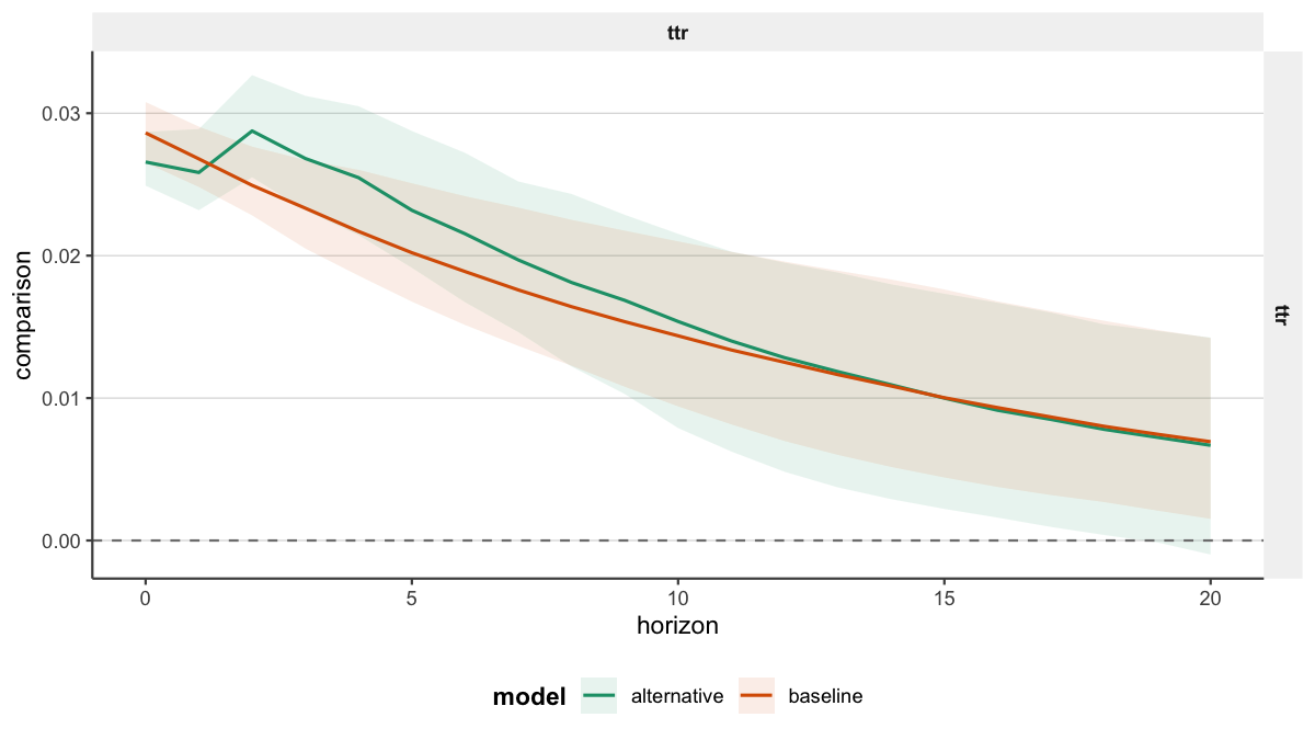
To evaluate sensitivity to the lag order, compare_irf() computes posterior summaries for both model specifications in a single table. Named arguments identify the specifications, while the remaining columns have the same meaning as in tidy_irf().

comparison <- compare_irf(
  baseline = post,
  longer_lag = post_alt,
  horizon = 12,
  probability = 0.90
)

subset(
  comparison,
  variable == "gdp" & shock == "gs" & horizon %in% c(0, 4, 8, 12),
  select = c(model, horizon, median, lower, upper))
#> # A tibble: 8 × 5
#>   model      horizon     median    lower    upper
#>   <chr>        <dbl>      <dbl>    <dbl>    <dbl>
#> 1 baseline         0 -0.0000935 -0.00115 0.000901
#> 2 baseline         4 -0.000702  -0.00191 0.000522
#> 3 baseline         8 -0.00119   -0.00301 0.000284
#> 4 baseline        12 -0.00158   -0.00394 0.000289
#> 5 longer_lag       0 -0.000111  -0.00117 0.000898
#> 6 longer_lag       4 -0.00100   -0.00316 0.00185 
#> 7 longer_lag       8 -0.00163   -0.00453 0.00206 
#> 8 longer_lag      12 -0.00220   -0.00544 0.00227

Differences in posterior medians or credible intervals indicate sensitivity to the model specification; they do not constitute a formal model-selection criterion. Corresponding comparisons are available for CDMs, FEVDs, forecasts, and historical-decomposition events.

How much posterior support does a statement have?

Pointwise support

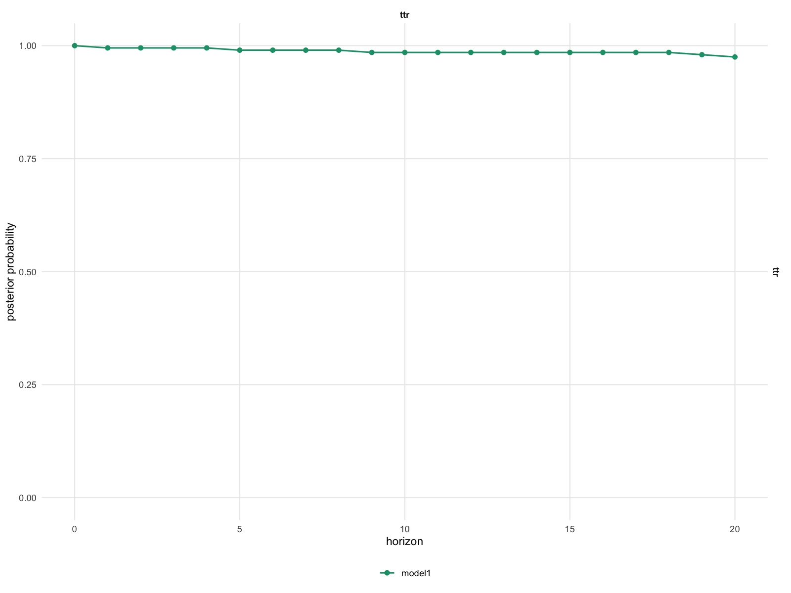
For a hypothesis at selected horizons, hypothesis_irf() reports the proportion of posterior draws that satisfy the stated inequality. Here the hypothesis is that the response of GDP is positive.

positive_gdp <- hypothesis_irf(
  post,
  variables = "gdp",
  shocks = "gs",
  horizon = c(0, 4, 8, 12),
  relation = ">",
  value = 0
)

positive_gdp[, c("horizon", "posterior_prob", "median_gap",
                 "lower_gap", "upper_gap")]
#> # A tibble: 4 × 5
#>   horizon posterior_prob median_gap lower_gap upper_gap
#>     <dbl>          <dbl>      <dbl>     <dbl>     <dbl>
#> 1       0          0.47  -0.0000935  -0.00115  0.000901
#> 2       4          0.185 -0.000702   -0.00191  0.000522
#> 3       8          0.11  -0.00119    -0.00301  0.000284
#> 4      12          0.09  -0.00158    -0.00394  0.000289

posterior_prob is the posterior probability of the stated inequality, conditional on the model specification; it is not a p-value. The gap columns summarise the posterior distribution of the response minus the threshold and therefore retain information about the magnitude of the response. Use hypothesis_cdm() for the same question about cumulative responses.

Joint support across a path

Pointwise probabilities do not give the probability that all conditions are satisfied simultaneously. For the stronger hypothesis that the response is positive from impact through horizon 8, joint_hypothesis_irf() evaluates the intersection of the nine inequalities within each posterior draw.

positive_path <- joint_hypothesis_irf(
  post,
  variable = "gdp",
  shock = "gs",
  horizon = 0:8,
  relation = ">",
  value = 0
)

positive_path[, c("posterior_prob", "n_constraints")]
#> # A tibble: 1 × 2
#>   posterior_prob n_constraints
#>            <dbl>         <int>
#> 1          0.095             9

The joint posterior probability can be considerably smaller than its pointwise counterparts because all nine inequalities must hold in the same posterior draw. See joint_hypothesis_cdm() for cumulative paths.

A magnitude question

A hypothesis about the sign alone may not address the economically relevant magnitude. Suppose 0.001 is a prespecified, substantively meaningful response on the scale used to estimate the model. magnitude_audit() reports the posterior probability that the absolute response exceeds this threshold at horizon 8.

material_response <- magnitude_audit(
  post,
  type = "irf",
  variable = "gdp",
  shock = "gs",
  horizon = 8,
  relation = ">",
  value = 0.001,
  absolute = TRUE
)

material_response[, c("posterior_prob", "median_gap",
                       "lower_gap", "upper_gap")]
#> # A tibble: 1 × 4
#>   posterior_prob median_gap lower_gap upper_gap
#>            <dbl>      <dbl>     <dbl>     <dbl>
#> 1          0.595   0.000229 -0.000818   0.00201

The threshold should follow from the variable transformation and the empirical application, and should not be selected from the posterior results. To evaluate cumulative dynamic multipliers, set type = "cdm"; the available scaling options are documented in magnitude_audit().

Does an interval cover the whole path?

Ordinary credible intervals have pointwise coverage. A 90% simultaneous credible band uses a single sup-norm critical value for the selected response path, so that 90% of posterior draws lie within the band over the complete selection.

gdp_band <- simultaneous_irf(
  post,
  horizon = 12,
  probability = 0.90,
  variables = "gdp",
  shocks = "gs"
)

gdp_band[gdp_band$horizon %in% c(0, 4, 8, 12),
         c("horizon", "median", "lower", "upper", "simultaneous_prob")]
#> # A tibble: 4 × 5
#>   horizon     median    lower    upper simultaneous_prob
#>     <dbl>      <dbl>    <dbl>    <dbl>             <dbl>
#> 1       0 -0.0000935 -0.00219 0.00201                0.9
#> 2       4 -0.000702  -0.00280 0.00140                0.9
#> 3       8 -0.00119   -0.00329 0.000914               0.9
#> 4      12 -0.00158   -0.00368 0.000523               0.9

The band applies only to the response variables, structural shocks, and horizons used in its construction. Expanding this set generally widens the band. Use simultaneous_cdm() for cumulative responses and plot_simultaneous() when a graphical representation facilitates interpretation of the response path.

Which single draw represents the posterior center?

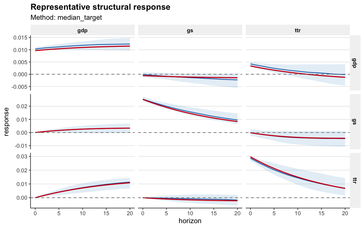
A response path formed from pointwise posterior medians need not correspond to any retained parameter draw. median_target_irf() instead selects the draw closest to the median target over the specified responses and horizons. Including both GDP and government spending in the target ensures that the two reported paths correspond to the same structural model draw.

representative <- median_target_irf(
  post, horizon = 12,
  variables = c("gdp", "gs"),
  shocks = "gs", horizons = 0:12
)

representative$draw_index
#> [1] 70

rep_path <- summary(representative)
subset(
  rep_path,
  variable == "gdp" & shock == "gs" & horizon %in% c(0, 4, 8, 12),
  select = c(horizon, median, draw_index, method))
#> # A tibble: 4 × 4
#>   horizon    median draw_index method       
#>     <dbl>     <dbl>      <int> <chr>        
#> 1       0 -0.000268         70 median_target
#> 2       4 -0.000827         70 median_target
#> 3       8 -0.00131          70 median_target
#> 4      12 -0.00172          70 median_target

This draw is appropriate when a subsequent calculation requires one internally consistent structural model. It is a representative draw, not a measure of posterior uncertainty; the full posterior distribution and its credible intervals should also be reported. The same selection is available for CDMs. For sign-restricted models, a distinct most-likely admissible draw can be selected.

When does the response arrive and fade?

The response-timing functions compute the relevant quantity for each posterior draw before summarising its distribution. Consequently, uncertainty about timing is not inferred from a single posterior median response. As an example of persistence, consider the response of government spending to its own shock over 20 quarters.

peak <- peak_response(post, horizon = 20, variables = "gs", shocks = "gs",
                      absolute = TRUE)
duration <- duration_response(
  post, horizon = 20, variables = "gs", shocks = "gs",
  relation = ">", value = 0, mode = "consecutive")
half_life <- half_life_response(
  post, horizon = 20, variables = "gs", shocks = "gs", baseline = "peak")
threshold <- time_to_threshold(
  post, horizon = 20, variables = "gs", shocks = "gs",
  relation = "<", value = 0.015)

data.frame(
  question = c("absolute peak", "positive spell", "half-life", "below 0.015"),
  posterior_median = c(
    peak$median_horizon,
    duration$median_duration,
    half_life$median_half_life,
    threshold$median_horizon
  ),
  unit = c("horizon", "periods", "periods after peak", "horizon"),
  reached_prob = c(NA, NA, half_life$reached_prob, threshold$reached_prob)
)
#>         question posterior_median               unit reached_prob
#> 1  absolute peak                0            horizon           NA
#> 2 positive spell               21            periods           NA
#> 3      half-life               14 periods after peak        0.900
#> 4    below 0.015               11            horizon        0.975

For half-life and threshold summaries, reached_prob is the posterior probability that the event occurs within the selected horizon. A conditional median may appear precise even when this probability is small. peak_response() also reports the posterior distribution of the peak value. Alternative definitions are documented for duration_response(), half_life_response(), and time_to_threshold().

Choose the statement that matches the question

• Use compare_*() to evaluate sensitivity across model specifications.
• Use hypothesis_*() to compute pointwise posterior probabilities.
• Use joint_hypothesis_*() when all selected inequalities must hold simultaneously.
• Use magnitude_audit() to evaluate a prespecified, economically relevant threshold.
• Use simultaneous_*() when the inferential statement concerns coverage of an entire selected response path.
• Use a median-target draw only when one coherent retained model draw is required.
• Use response-timing summaries to report when, for how long, and with what probability a response reaches a specified event; these summaries do not replace the posterior distribution of the response.

For posterior diagnostics and representative draws in sign-restricted models, see Analysis of Sign-Restricted Models. The reference index documents related variants and plotting methods.