Analysis of Sign-Restricted Models

This article considers a PosteriorBSVARSIGN object estimated with bsvarSIGNs. It assumes familiarity with the specification of sign, zero, structural, and narrative restrictions. The analysis addresses three distinct questions: the selection of a representative admissible draw, the posterior probability that each restriction is satisfied, and the adequacy of the stored posterior sample.

These are three different questions:

Question	Function	What the result means
Which admissible draw is representative of the posterior distribution?	most_likely_admissible_irf() or most_likely_admissible_cdm()	One posterior draw selected according to its admissibility weight
What is the posterior probability that each restriction is satisfied?	restriction_audit()	Posterior satisfaction probability for each fitted restriction
Does the stored sample contain sufficient effective information and admissibility support?	acceptance_diagnostics()	Effective sample size (ESS), search settings, restriction counts, and the distribution of admissibility weights

These quantities have different interpretations. A representative draw does not establish that every restriction has high posterior support. Conversely, a high satisfaction probability does not establish that the effective sample size is large or that the admissibility weights are sufficiently dispersed.

Posterior input

The following example uses the optimism data from bsvarSIGNs. The code specifies the identifying restrictions and estimates the posterior distribution. In an empirical application, post_sign can be replaced by any fitted PosteriorBSVARSIGN object.

data("optimism", package = "bsvarSIGNs")

sign_irf <- matrix(c(0, 1, rep(NA_real_, 23)), 5, 5)
spec_sign <- bsvarSIGNs::specify_bsvarSIGN$new(optimism * 100, p = 4,
  sign_irf = sign_irf)

set.seed(123)
post_sign <- bsvars::estimate(spec_sign, S = 2000, thin = 1,
  show_progress = FALSE)

The remaining examples are not evaluated because the package does not include a precomputed sign-restricted posterior. They can be evaluated after fitting the model above.

Select a representative admissible draw

most_likely_admissible_irf() ranks the posterior draws according to the admissibility kernel of the fitted sign-restricted model. If several draws have the highest weight, the function selects the draw closest to the posterior median response path. The result is one internally coherent posterior draw, rather than a path assembled from marginal quantiles.

rep_irf <- most_likely_admissible_irf(post_sign, horizon = 12)

rep_irf$draw_index
rep_irf$score

rep_path <- subset(summary(rep_irf),
  variable == "productivity" & shock == "productivity" &
    horizon %in% c(0, 4, 8, 12),
  select = c(variable, shock, horizon, median, draw_index, method, score))
rep_path

plot() compares the selected path with the pointwise posterior summary. The red path represents the selected posterior draw; it is neither an additional credible interval nor a model-selection result.

plot(rep_irf)

most_likely_admissible_cdm() applies the same selection rule to cumulative dynamic responses computed separately for each posterior draw:

rep_cdm <- most_likely_admissible_cdm(post_sign, horizon = 12)
summary(rep_cdm)
plot(rep_cdm)

The choice between the IRF and CDM functions depends on whether impulse or cumulative responses are of substantive interest. The posterior draws selected by the two criteria need not be identical.

Evaluate restriction satisfaction

For a PosteriorBSVARSIGN object, restriction_audit() extracts the impulse- response, zero, structural, and narrative restrictions from the identification scheme. It reports the posterior probability that each restriction is satisfied, estimated by the proportion of stored posterior draws that satisfy the restriction.

audit <- restriction_audit(post_sign, zero_tol = 1e-6)
audit_focus <- audit[, c("restriction_type", "restriction", "relation",
                         "posterior_prob")]
audit_focus

zero_tol defines the numerical tolerance used to evaluate a zero restriction. Its value should reflect the scale of the response and should be reported when zero restrictions are included.

plot_restriction_audit() visualises the posterior satisfaction probabilities. Formatted labels improve legibility without changing the underlying restriction definitions.

plot_restriction_audit(audit, label_style = "pretty",
  restriction_types = c("irf_sign", "irf_zero"))

The reported probabilities are conditional on the fitted posterior distribution and the chosen tolerance. They are not sampler acceptance rates and do not measure whether admissible draws are concentrated in a small region of the parameter space.

Assess the stored posterior sample

acceptance_diagnostics() reports properties available from the stored posterior distribution: the number of draws, effective sample size, max_tries, restriction counts, and the distribution of admissibility weights.

diag <- acceptance_diagnostics(post_sign, ess_threshold = 100,
  sparse_threshold = 0.10)

subset(diag,
  metric %in% c(
    "posterior_draws", "effective_sample_size", "max_tries",
    "kernel_zero_share", "kernel_cv"),
  select = c(metric, value, flag, message))

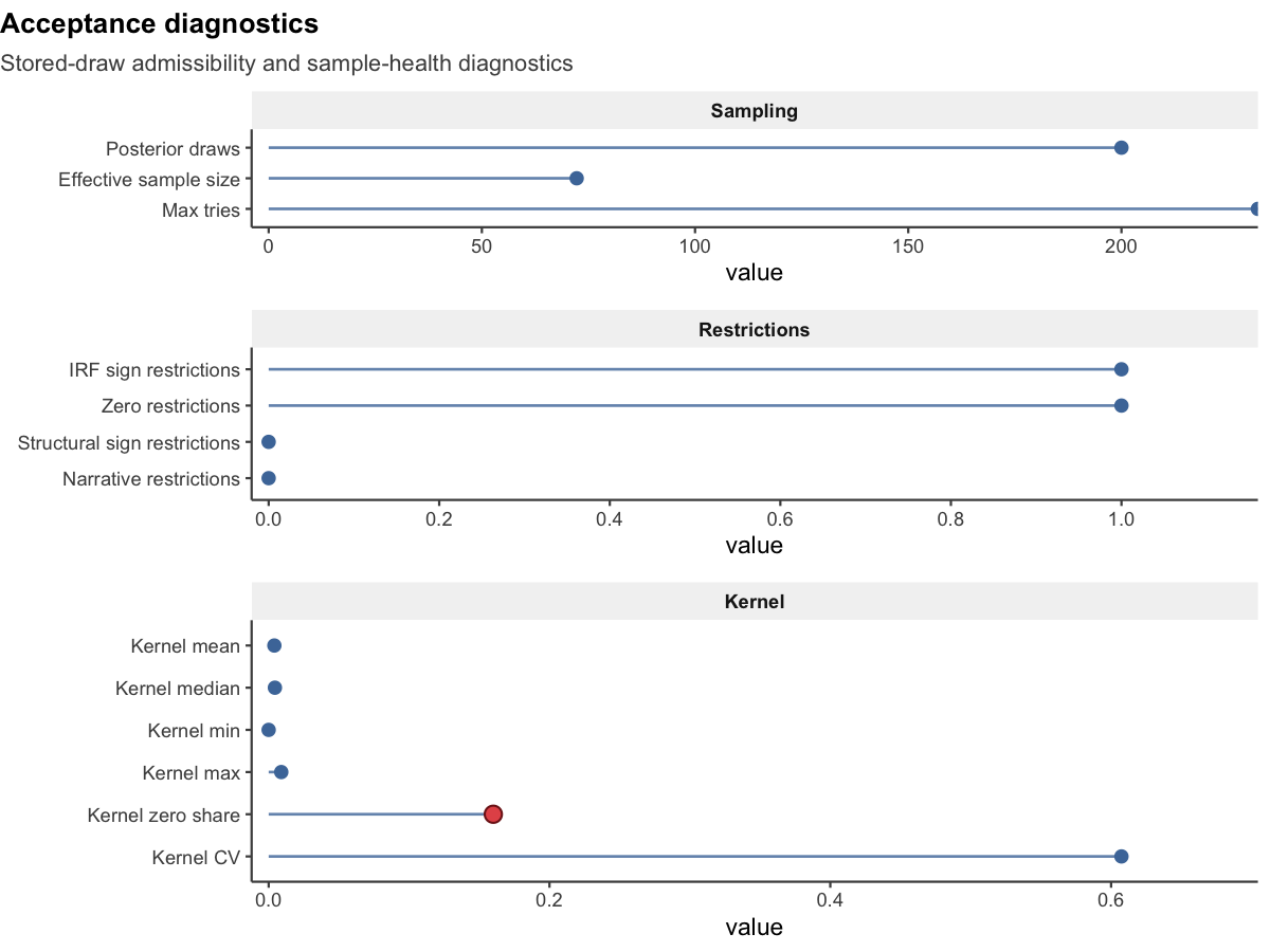
effective_sample_size measures the effective amount of posterior information, while kernel_zero_share reports the proportion of near-zero admissibility weights. kernel_cv measures the dispersion of these weights. The restriction counts and max_tries indicate the computational demands of the identification search.

The specified thresholds identify potentially weak effective information or sparse admissibility support; they are not universal decision rules. These diagnostics cannot recover the sampler’s complete proposal and rejection history from the stored posterior distribution.

The following figure illustrates the diagnostic measures for a posterior from the sign-restricted specification above with 200 retained draws.

plot_acceptance_diagnostics(diag,
  metrics = c("effective_sample_size", "kernel_zero_share", "kernel_cv"),
  title = "Stored-sample diagnostics")

Examine shock contributions over a selected period

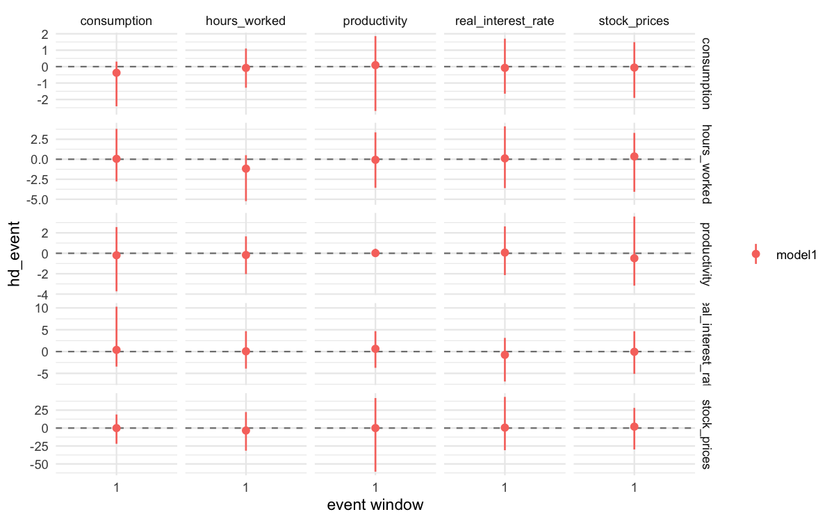
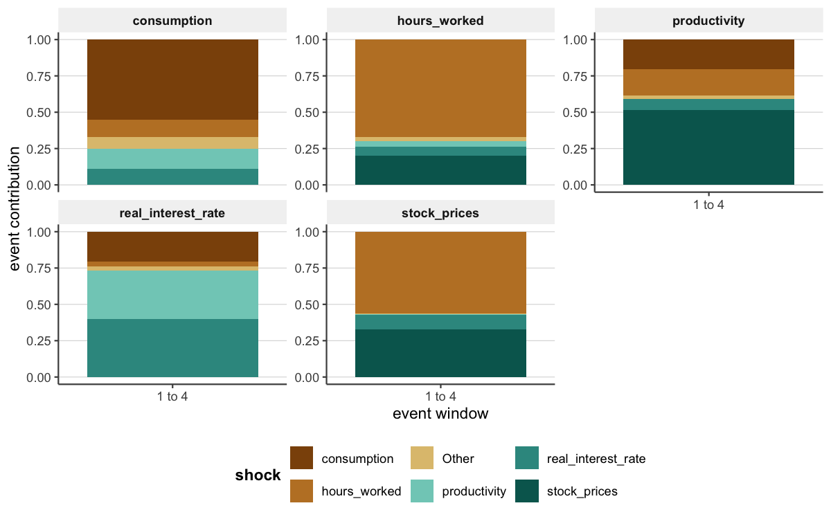
Historical decompositions from a sign-restricted posterior can be summarised over a prespecified period in the same way as other supported posterior objects. The figures below show posterior contributions and their proportional composition over observations 1 to 4 for the illustrative specification.

Compare sign-restricted specifications

Alternative specifications should contain the same variables and comparable identifying restrictions. Names assigned to the posterior arguments identify the specifications in the comparison tables.

spec_sign_alt <- bsvarSIGNs::specify_bsvarSIGN$new(optimism * 100, p = 2,
  sign_irf = sign_irf)

set.seed(456)
post_sign_alt <- bsvars::estimate(spec_sign_alt, S = 2000, thin = 1,
  show_progress = FALSE)

Posterior restriction probabilities and sample diagnostics are compared separately:

restriction_comparison <- compare_restrictions(baseline = post_sign,
  shorter_lag = post_sign_alt, zero_tol = 1e-6)

diagnostic_comparison <- compare_acceptance_diagnostics(
  baseline = post_sign,
  shorter_lag = post_sign_alt,
  ess_threshold = 100,
  sparse_threshold = 0.10)

compare_restrictions() reports posterior satisfaction probabilities by model, whereas compare_acceptance_diagnostics() reports the corresponding diagnostic measures. Differences in either table describe fitted posterior distributions and stored samples; they do not, by themselves, rank the economic plausibility of the specifications.

plot_compare_restrictions(restriction_comparison,
  restriction_types = c("irf_sign", "irf_zero"))

plot_acceptance_diagnostics(
  diagnostic_comparison,
  metrics = c("effective_sample_size", "kernel_zero_share", "kernel_cv"))

Recommended sequence of analysis

For each reported sign-restricted result:

1. Evaluate the effective sample size and admissibility-weight distribution with acceptance_diagnostics() before interpreting posterior summaries.
2. Use restriction_audit() to report the posterior satisfaction probabilities of the fitted restrictions.
3. Select a most-likely-admissible IRF or CDM only when one coherent draw is required for presentation or subsequent calculations.
4. Compare diagnostics and restriction probabilities across substantively relevant alternative specifications rather than comparing representative paths alone.

For posterior summaries, probability statements, response timing, figures, and tables, see Post-estimation Analysis with bsvarPost. The function reference documents filters, tolerances, and plotting arguments.