Historical-Decomposition Analysis

Historical decompositions from bsvars and bsvarSIGNs describe the contributions of structural shocks to observed variables through time. bsvarPost summarises these contributions over a substantively chosen period, ranks the shocks within that period, and compares the same event across model specifications.

This article assumes that you already have a fitted posterior and understand the identification behind its shock labels. See the parent-package documentation for estimation and the standard historical-decomposition analysis. The precomputed fiscal posteriors used here avoid re-estimation and make the numerical results reproducible.

Posterior draws of shock contributions

Event-specific summaries require posterior draws rather than a table of pointwise posterior intervals. Obtain the draw-level contributions with tidy_hd(draws = TRUE):

hd_draws <- tidy_hd(post, draws = TRUE)

data.frame(
  first = head(unique(as.character(hd_draws$time)), 1),
  last = tail(unique(as.character(hd_draws$time)), 1),
  draws = length(unique(hd_draws$draw))
)
#>     first    last draws
#> 1 1948.25 2024.25   200

Each row identifies a model, variable, shock, observation, and posterior draw. Retaining the draws ensures that posterior uncertainty is summarised after the contributions have been aggregated over the selected period.

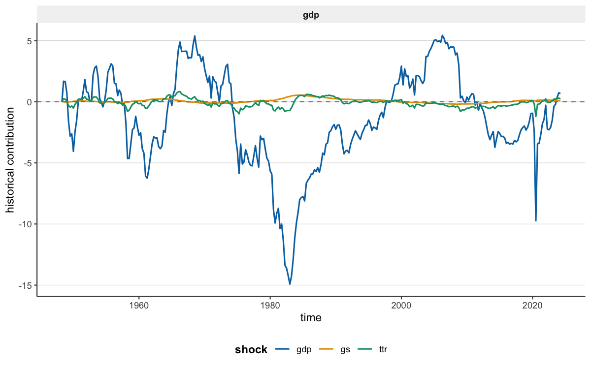
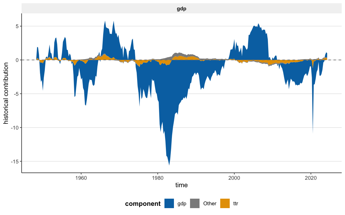
The full-sample decomposition provides context for selecting an event period. The first figure displays the principal shock contributions separately; the second displays their composition.

Define the event period before ranking shocks

The event period is determined by the empirical question rather than by the estimated ranking of shocks. A defensible analysis therefore usually does three things:

1. Define the dates from the research question or an external chronology, before inspecting which shock ranks first.
2. Match start and end to the model’s time labels and use a window consistent with the data frequency.
3. Repeat the analysis over reasonable neighboring windows as a sensitivity check, without silently replacing the prespecified result.

For this example, we use the complete four-quarter period from 1958 to 1958.75. It is a convenient interval covered by both stored posterior samples; the example does not assign a particular historical interpretation to this period. The samples contain only 200 posterior draws, and the interpretation of the shock names follows from the identification of the fitted model.

event_start <- "1958"
event_end <- "1958.75"

event <- tidy_hd_event(
  hd_draws,
  start = event_start,
  end = event_end,
  probability = 0.90
)

subset(
  event,
  variable == "gdp",
  select = c(variable, shock, event_start, event_end,
             median, lower, upper)
)
#> # A tibble: 3 × 7
#>   variable shock event_start event_end median  lower  upper
#>   <chr>    <chr> <chr>       <chr>      <dbl>  <dbl>  <dbl>
#> 1 gdp      gdp   1958        1958.75   -14.9  -53.5  24.4  
#> 2 gdp      gs    1958        1958.75    -3.15 -11.9   0.435
#> 3 gdp      ttr   1958        1958.75    -1.23  -5.86  4.48

tidy_hd_event() sums each shock’s contribution across the inclusive period separately for each posterior draw, then reports posterior summaries. Set draws = TRUE when a subsequent calculation requires the aggregated draws themselves.

The largest posterior median should not be interpreted as certainty about a shock’s historical importance. The interval columns report posterior uncertainty, while the structural interpretation of each shock follows from the identification of the original model.

Rank shock contributions

shock_ranking() orders shocks separately within each model-variable panel. Restricting to gdp keeps the result aligned with one research question.

ranking <- shock_ranking(
  hd_draws,
  start = event_start,
  end = event_end,
  variables = "gdp",
  ranking = "absolute",
  probability = 0.90
)

ranking[, c("variable", "shock", "median", "lower", "upper", "rank")]
#> # A tibble: 3 × 6
#>   variable shock median  lower  upper  rank
#>   <chr>    <chr>  <dbl>  <dbl>  <dbl> <int>
#> 1 gdp      gdp   -14.9  -53.5  24.4       1
#> 2 gdp      gs     -3.15 -11.9   0.435     2
#> 3 gdp      ttr    -1.23  -5.86  4.48      3

ranking = "absolute" answers which shock has the largest median contribution in absolute value. Use ranking = "signed" when the direction of the contribution is part of the estimand. In either case, rank summarises the posterior median; overlapping credible intervals may indicate substantial uncertainty about the ordering.

The ranked-contribution plot displays the sign and scale of each contribution while ordering the bars by the absolute posterior median.

ranking_plot <- publish_bsvar_plot(
  ranking,
  family = "shock_ranking",
  preset = "paper",
  title = "GDP contributions during the selected window",
  caption = "Bars are posterior medians; uncertainty remains in the event table."
)
ranking_plot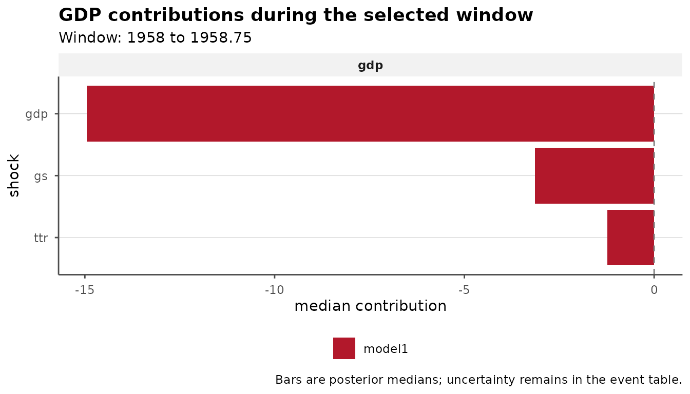

To visualise contributions without ranking them, use plot_hd_event(). The more specialized plot_hd_event_share(), plot_hd_event_cumulative(), and plot_hd_event_distribution() report the composition of contributions, their accumulation within the selected period, and their posterior distributions, respectively.

Compare the same event across specifications

When assessing sensitivity to the lag order or prior distribution, the event definition should remain fixed. compare_hd_event() applies the same period to named posterior objects and returns estimates indexed by model specification.

event_comparison <- compare_hd_event(
  baseline = post,
  alternative = post_alt,
  start = event_start,
  end = event_end,
  probability = 0.90
)

comparison_gdp <- subset(
  event_comparison,
  variable == "gdp",
  select = c(model, shock, event_start, event_end,
             median, lower, upper)
)
comparison_gdp
#> # A tibble: 6 × 7
#>   model       shock event_start event_end    median  lower  upper
#>   <chr>       <chr> <chr>       <chr>         <dbl>  <dbl>  <dbl>
#> 1 baseline    gdp   1958        1958.75   -14.9     -53.5  24.4  
#> 2 baseline    gs    1958        1958.75    -3.15    -11.9   0.435
#> 3 baseline    ttr   1958        1958.75    -1.23     -5.86  4.48 
#> 4 alternative gdp   1958        1958.75   -19.1     -51.5  17.0  
#> 5 alternative gs    1958        1958.75    -0.00276  -6.11  3.89 
#> 6 alternative ttr   1958        1958.75    -1.62     -6.60  4.49

This comparison is descriptive. Similar estimates across specifications provide evidence of robustness, but compare_hd_event() neither selects a preferred model nor computes the posterior probability that the specifications differ. When comparing additional periods, retain names such as baseline and alternative to identify each specification in tables and figures.

Report posterior summaries

The comparison can be reported in a labelled table, and the ranked-contribution plot can be saved separately. Both objects remain standard R objects, so captions, annotations, and journal-specific formatting can be added as needed.

as_kable(
  comparison_gdp,
  caption = "GDP shock contributions in the selected event window",
  digits = 2,
  preset = "compact"
)

GDP shock contributions in the selected event window

Model	Shock	Event start	Event end	Median	Lower	Upper
baseline	gdp	1958	1958.75	-14.95	-53.50	24.36
baseline	gs	1958	1958.75	-3.15	-11.87	0.43
baseline	ttr	1958	1958.75	-1.23	-5.86	4.48
alternative	gdp	1958	1958.75	-19.05	-51.50	16.99
alternative	gs	1958	1958.75	0.00	-6.11	3.89
alternative	ttr	1958	1958.75	-1.62	-6.60	4.49

ggplot2::ggsave(
  "shock-ranking-1958.pdf",
  ranking_plot,
  width = 7,
  height = 4
)

For an introduction to posterior summaries, response comparisons, and posterior probability statements, see Post-estimation Analysis with bsvarPost. For diagnostics specific to sign-restricted identification, continue to the dedicated bsvarSIGNs article.